Geographically Weighted Regression on Indonesian Human Development Index in 2024 (Part 2)

This article is a continuation from results part of previous article. The processing steps done from previous article are:

1. Importing the data of HDI into R
2. Importing the provincial shapefile and HDI dataset into R.
3. Doing the statistics descriptive with histogram etc.
4. Merging attribute data with spatial geometries using a left join operation.

In this article, we continue the steps:

1. Doing the Linear Regression OLS model
2. Multicolinearity test, Normality test, Heteroscedasticity test, Non autocorrelation test

Results and Discussions

We do the Linear Regression OLS Model at first to create a Global model. Next we test if the model has the spatial heterogeneity to be done with Geographically Weighted Regression model.

ipmlm <- lm(y ~ (x1+x3+x5+x6),data=hdi)
summary(ipmlm)

result:
Call:
lm(formula = y ~ (x1 + x3 + x5 + x6), data = hdi)

Residuals:
    Min      1Q  Median      3Q     Max 
-4.7905 -0.9212 -0.2494  1.0178  5.2864 

Coefficients:
              Estimate Std. Error t value Pr(>|t|)    
(Intercept)  4.687e+01  3.403e+00  13.774 3.08e-15 ***
x1           2.366e-06  7.326e-07   3.230   0.0028 ** 
x3           2.150e-01  3.778e-02   5.692 2.39e-06 ***
x5          -1.639e-01  7.613e-02  -2.152   0.0388 *  
x6           2.484e+00  1.071e+00   2.319   0.0267 *  
---
Signif. codes:  0 ‘***’ 0.001 ‘**’ 0.01 ‘*’ 0.05 ‘.’ 0.1 ‘ ’ 1

Residual standard error: 2.182 on 33 degrees of freedom
Multiple R-squared:  0.8399,	Adjusted R-squared:  0.8204 
F-statistic: 43.27 on 4 and 33 DF,  p-value: 1.113e-12   

Statistical Diagnostics
Perform statistical diagnostics to check whether the model has spatial effects or spatial heterogeneity.

par(mfrow=c(2,2))
plot(ipmlm) 

Multicollinearity Test
Multicollinearity testing is indicated by the VIF value. A relationship between predictor variables in a multiple linear regression model is indicated when the VIF value is >10. If the VIF value for each predictor variable is less than 10, it can be concluded that there is no multicollinearity between the predictor variables.

library(car)
vif(ipmlm)

result:
      x1       x3       x5       x6 
1.169276 2.518185 3.538650 2.119537 

Correlation Plot
Create correlation plot of all variables

library(corrplot)
cordata = cor(hdi1)
corrplot(cordata,method = 'number')

Normality Test
Hypothesis
H0: Data is normally distributed
H1: Data is not normally distributed
Test Criteria
Reject H0 if p-value <0.05 Sample <50, use the Sapphiro test; if n>50, use the Kolmogorov-Smirnov test.

resids <- residuals(ipmlm)
shapiro.test(resids)

result:
	Shapiro-Wilk normality test

data:  resids
W = 0.98111, p-value = 0.7566

HETEROKEDASTICITY TEST
Hypothesis
H0: Homoscedasticity
H1: Heteroscedasticity
Test Criteria
Reject H0 if p-value < alpha. (significant)

library(lmtest)
bptest(ipmlm)

result:
	studentized Breusch-Pagan test

data:  ipmlm
BP = 1.7996, df = 4, p-value = 0.7726

NON-AUTOCORRELATION TEST
Hypothesis
H0: Data is non-autocorrelated
H1: Data is autocorrelated
Test Criteria
Reject H0 if p-value < alpha

durbinWatsonTest(ipmlm)

result:
 lag Autocorrelation D-W Statistic p-value
   1     -0.07633825      2.098435   0.908
 Alternative hypothesis: rho != 0

Establishing the spatial weighting matrix (W)
The previous regression did not consider spatial elements in its analysis. Therefore, we will test for spatial autocorrelation using Moran’s Test. To do this, we first need to find and calculate the spatial weights.

K-nearest neighboard

coords <- st_coordinates(st_centroid(map_prov))
coords <- coords[,1:2]
head(coords)

result:
            X          Y
[1,] 121.1620 -1.0104509
[2,] 119.3504 -2.4546476
[3,] 120.1605 -3.6888069
[4,] 136.6159 -3.9097732
[5,] 133.6419 -2.6539586
[6,] 122.3600  0.6954182

W.knn<-knn2nb(knearneigh(coords, k=5 ,longlat=TRUE))
W.knn1 <- nb2listw(W.knn,style='W') 
W.knn1

Inverse distance

distance_matrix <- as.matrix(dist(coords, method="euclidean"))
inv_dist <- 1/distance_matrix
diag(inv_dist) <- 0
W.id<-mat2listw(inv_dist, style="W")
summary(W.id)

Rook Contiguity

W.rook <- poly2nb(map_prov_hdi, row.names=map_prov_hdi$id, queen=FALSE)
W.rook.s <- nb2listw(W.rook,style='B', zero.policy = TRUE) ; 
W.rook.s

Queen Contiguity

W.queen <- poly2nb(map_prov, row.names=map_prov$id, queen=TRUE)
W.queen.s <- nb2listw(W.queen,style='B', zero.policy = TRUE) ; W.queen.s

Choosing spatial weights

MI.knn <- moran(ipm1$y, W.knn1, n=length(W.knn1$neighbours), S0=Szero(W.knn1))
MI.id <- moran(ipm1$y, W.id, n=length(W.id$neighbours), S0=Szero(W.id))
MI.rook <- moran.test(ipm1$y, W.rook.s, randomisation = TRUE, zero.policy = TRUE)
MI.queen <- moran.test(ipm1$y, W.queen.s, randomisation = TRUE, zero.policy = TRUE)
moran_index<-data.frame(
  "Weight matrix"=c("KNN (k=5)", "Inverse distance weight", "Rook Contiguity", "Queen Contiguity"),
  "Moran's I"=c(MI.knn$I, MI.id$I, 0.22785882,0.22785882 ))
moran_index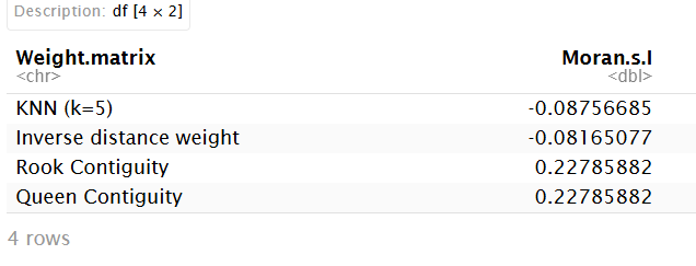

Checking for spatial effects using the Moran’s I test, we get the largest Moran’s I is Rook Contiguity.
Optimum W
The optimal weight is selected based on the largest Moran’s I statistic.

W_optimum <- W.rook.s
moran.test(ipm1$y,W_optimum)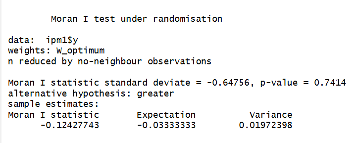

par(mar = c(5, 5, 2, 2))
moran.plot(ipm1$y, W_optimum, labels=ipm1$id)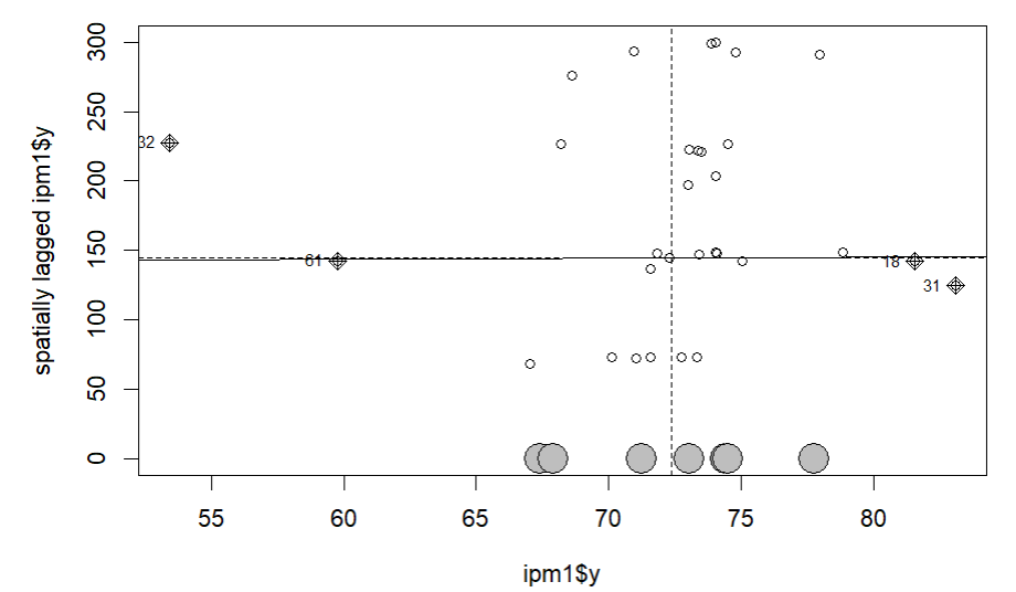

Continue to Geographically Weighted Regression on Indonesian Human Development Index in 2024 (Part 3).