Spatial autocorrelation refers to the degree to which nearby geographic observations are similar or dissimilar to each other.

In simple terms:

Spatial autocorrelation measures whether spatial patterns are clustered, dispersed, or random.

It is one of the most fundamental concepts in:

• GIS,
• spatial statistics,
• spatial econometrics,
• geography,
• spatial data science.

---

Why Spatial Autocorrelation Matters

Traditional statistical methods assume that observations are independent.

However, spatial data often violates this assumption because nearby locations tend to influence one another.

Examples:

• neighboring districts often have similar income levels,
• nearby houses tend to have similar prices,
• adjacent regions may share similar climate conditions,
• disease outbreaks often cluster geographically.

This phenomenon is known as spatial dependence.

---

Tobler’s First Law of Geography

Spatial autocorrelation is closely related to:

“Everything is related to everything else, but near things are more related than distant things.”

— Waldo Tobler

This principle explains why spatial autocorrelation exists in many real-world phenomena.

---

Types of Spatial Autocorrelation

There are three major patterns:

Type	Meaning
Positive Spatial Autocorrelation	Nearby values are similar
Negative Spatial Autocorrelation	Nearby values are dissimilar
Zero Spatial Autocorrelation	Spatial randomness

---

1. Positive Spatial Autocorrelation

High values tend to be near high values, and low values near low values.

Example:

• expensive houses cluster together,
• high-income neighborhoods are adjacent.

---

Positive Spatial Autocorrelation Example

5

---

2. Negative Spatial Autocorrelation

High values tend to be near low values.

Example:

• checkerboard-like patterns,
• alternating land-use zones.

---

Negative Spatial Autocorrelation Example

7

---

3. No Spatial Autocorrelation

Spatial patterns appear random.

Nearby observations do not show systematic similarity.

---

Random Spatial Pattern Example

7

---

Why Spatial Autocorrelation Is Important

Spatial autocorrelation affects:

• statistical inference,
• regression models,
• prediction accuracy,
• hypothesis testing.

Ignoring spatial autocorrelation can lead to:

• biased standard errors,
• misleading significance tests,
• incorrect conclusions.

---

Global vs Local Spatial Autocorrelation

Spatial autocorrelation can be analyzed at two levels.

Type	Purpose
Global Spatial Autocorrelation	Measures overall spatial pattern
Local Spatial Autocorrelation	Detects local clusters and hotspots

---

Global Spatial Autocorrelation

Global measures summarize the overall spatial pattern of an entire study area.

The most famous method is:

Moran’s I

---

Moran’s I Formula

$I=\frac{n}{\sum_i\sum_j w_{ij}}\frac{\sum_i\sum_j w_{ij}(x_i-\bar{x})(x_j-\bar{x})}{\sum_i(x_i-\bar{x})^2}$I=∑i​∑j​wij​n​∑i​(xi​−xˉ)2∑i​∑j​wij​(xi​−xˉ)(xj​−xˉ)​

Where:

Symbol	Meaning
$n$n	Number of observations
$x_i$xi​	Value at location $i$i
$w_{ij}$wij​	Spatial weight between locations
$\bar{x}$xˉ	Mean value

---

Interpretation of Moran’s I

Moran’s I Value	Interpretation
$I > 0$I>0	Positive spatial autocorrelation
$I < 0$I<0	Negative spatial autocorrelation
$I \approx 0$I≈0	Spatial randomness

---

Spatial Weight Matrix

Spatial autocorrelation depends on defining neighborhood relationships.

This is represented using a spatial weight matrix.

Example:

• neighboring districts = 1,
• non-neighbors = 0.

---

Spatial Weight Matrix Illustration

6

---

Common Spatial Weight Methods

Method	Description
Contiguity-based	Shared boundaries
Distance-based	Based on geographic distance
k-Nearest Neighbor	Closest neighbors

---

Local Spatial Autocorrelation (LISA)

Local Indicators of Spatial Association (LISA) identify local clusters such as:

• hotspots,
• coldspots,
• spatial outliers.

---

LISA Cluster Types

Cluster	Meaning
High-High	High values surrounded by high values
Low-Low	Low values surrounded by low values
High-Low	Spatial outlier
Low-High	Spatial outlier

---

LISA Cluster Map Example

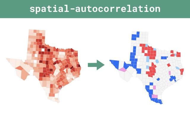
6

---

Applications of Spatial Autocorrelation

Spatial autocorrelation is widely used in:

Field	Example
Real Estate	House price clustering
Epidemiology	Disease hotspots
Urban Planning	Land-use patterns
Environmental Science	Pollution clustering
Transportation	Traffic congestion analysis
Agriculture	Soil variability

---

Spatial Autocorrelation in R

R provides powerful tools for spatial autocorrelation analysis.

Common packages:

• sf
• spdep
• tmap

---

Install Required Packages

install.packages(c("sf", "spdep"))

---

Load Packages

library(sf)library(spdep)

---

Read Spatial Data

data <- st_read("districts.shp")

---

Create Spatial Neighbors

neighbors <- poly2nb(data)

---

Convert to Spatial Weight Matrix

weights <- nb2listw(neighbors)

---

Compute Moran’s I

Suppose the variable is:

• poverty rate,
• house price,
• unemployment rate.

moran.test(data$poverty_rate, weights)

---

Example Output

Moran I statistic standard deviate = 4.82p-value = 0.00001Moran's I = 0.41

Interpretation:

• Moran’s I = 0.41
• positive spatial autocorrelation exists,
• nearby regions tend to have similar poverty rates.

---

Visualizing Spatial Autocorrelation

Moran Scatter Plot

moran.plot(data$poverty_rate, weights)

---

Moran Scatter Plot Example

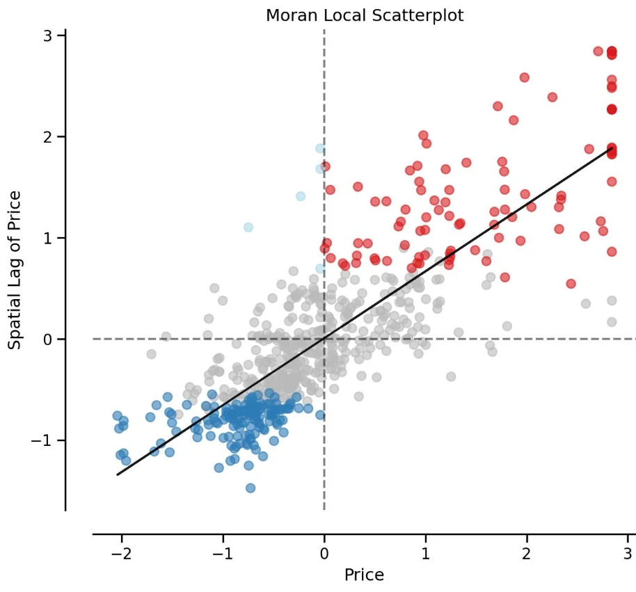
5

---

Mapping Local Moran’s I

local_moran <- localmoran(data$poverty_rate, weights)data$Ii <- local_moran[,1]plot(data["Ii"])

---

Spatial Autocorrelation and Regression

One major implication:

OLS regression assumptions may fail.

If residuals contain spatial autocorrelation:

• coefficients may remain unbiased,
• but inference becomes unreliable.

This motivates spatial regression models such as:

• Spatial Lag Model (SLM),
• Spatial Error Model (SEM),
• Geographically Weighted Regression (GWR).

---

Common Mistakes

1. Ignoring CRS

Spatial relationships depend on coordinate systems.

---

2. Using Incorrect Spatial Weights

Different neighbor definitions may produce different results.

---

3. Assuming Correlation Means Causation

Spatial clustering does not necessarily imply causal relationships.

---

Spatial Autocorrelation vs Traditional Correlation

Traditional Correlation	Spatial Autocorrelation
Relationship between variables	Relationship across space
No location information	Spatial location matters
Independent observations assumed	Spatial dependence considered

---

Conclusion

Spatial autocorrelation measures how strongly geographic observations relate across space.

It is one of the most important concepts in:

• GIS,
• spatial statistics,
• spatial econometrics,
• spatial data science.

Understanding spatial autocorrelation helps analysts:

• detect clustering,
• identify spatial patterns,
• improve regression models,
• avoid misleading statistical inference.

Methods such as Moran’s I and LISA have become essential tools for modern spatial analysis.