Spatial heterogeneity refers to the condition where relationships, patterns, or processes vary across geographic space. In simple terms:

A relationship observed in one location may not behave the same way in another location.

Spatial heterogeneity is one of the core concepts in:

• GIS,
• spatial statistics,
• spatial econometrics,
• spatial data science,
• geography.

Why Spatial Heterogeneity Matters

Many traditional statistical models assume:

• relationships are constant,
• parameters are globally fixed,
• one model applies equally everywhere.

However, real-world spatial processes are rarely uniform. Examples:

• the effect of distance to the city center on house prices differs between urban and rural areas,
• rainfall impacts agricultural productivity differently across regions,
• education may influence income differently across provinces,
• accessibility may affect land value differently between metropolitan and suburban areas.

These spatially varying relationships indicate spatial heterogeneity.

Spatial Heterogeneity vs Spatial Autocorrelation

Spatial heterogeneity and spatial autocorrelation are related but fundamentally different concepts.

Concept	Meaning
Spatial Autocorrelation	Nearby observations tend to be similar
Spatial Heterogeneity	Relationships vary across space

Spatial autocorrelation focuses on: similarity among neighboring observations. Spatial heterogeneity focuses on: variation in relationships or processes across locations.

Example of Spatial Heterogeneity

Suppose we model house prices using: house size, distance to the CBD.

A traditional regression model may be written as:

$Price=\beta_0+\beta_1(Size)+\beta_2(Distance)+\varepsilon$Price=β0​+β1​(Size)+β2​(Distance)+ε

This model assumes: $\beta_1$β1​ and $\beta_2$β2​ are constant everywhere.

In reality:

• distance to the CBD may strongly affect prices in dense urban areas,
• but have weak influence in rural regions.

This indicates that the relationship varies spatially.

Why Spatial Heterogeneity Occurs

Spatial heterogeneity arises because locations differ in:

• economic conditions,
• demographics,
• accessibility,
• infrastructure,
• environmental conditions,
• policy,
• land use,
• social behavior.

Geographic context changes how variables interact.

Types of Spatial Heterogeneity

Spatial heterogeneity can appear in several forms.

Type	Description
Structural Heterogeneity	Relationships differ spatially
Variance Heterogeneity	Variability differs across locations
Functional Heterogeneity	Different processes operate in different regions
Scale Heterogeneity	Relationships change across spatial scales

Structural Spatial Heterogeneity

Regression relationships vary geographically. Example:

• income may strongly influence housing prices in cities,
• but weakly influence prices in rural regions.

Variance Heterogeneity

The variability of observations differs spatially. Example:

• property prices may fluctuate heavily in downtown areas,
• but remain relatively stable in suburban zones.

Spatial Nonstationarity

Spatial heterogeneity is closely related to spatial nonstationarity. A spatial process is nonstationary when:

• statistical relationships change across geographic space.

Stationary vs Nonstationary Processes

Stationary Process	Nonstationary Process
Relationships constant	Relationships vary spatially
Global structure	Local variation
One model sufficient	Local analysis needed

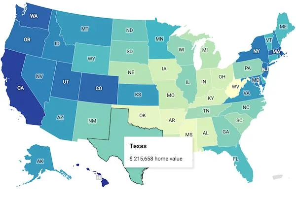
Visualization of Spatial Heterogeneity

Spatially Varying Relationship

Why Global Models May Be Problematic

Many global statistical models assume: $y=X\beta+\varepsilon$y=Xβ+ε

where: $\beta$β is constant across all locations.

When spatial heterogeneity exists:

• important local variation may be hidden,
• model accuracy may decline,
• local patterns may be oversimplified.

Detecting Spatial Heterogeneity

Several approaches can help identify spatial heterogeneity.

1. Residual Mapping

Spatially clustered residuals may indicate:

• missing local variation,
• unmodeled spatial processes.

Regional Comparison

Relationships can be compared across:

• cities,
• provinces,
• districts,
• spatial clusters.

Large differences may indicate spatial heterogeneity.

Exploratory Spatial Data Analysis (ESDA)

Spatial Heterogeneity in Real Estate

Spatial heterogeneity is especially important in property valuation.

Examples:

• proximity to public transportation may strongly increase property value in urban centers,
• but have limited effect in low-density suburban regions.

Similarly:

• school quality may strongly affect prices in some districts,
• but weakly affect prices elsewhere.

---

Spatial Heterogeneity in Environmental Studies

Examples include:

• rainfall effects varying by elevation,
• pollution behavior differing across industrial zones,
• climate impacts changing geographically.

---

Spatial Heterogeneity in Public Health

Examples:

• disease transmission differs across regions,
• healthcare accessibility varies spatially,
• socioeconomic factors influence health outcomes differently across cities.

---

Spatial Heterogeneity in R

R provides powerful tools for exploring spatial heterogeneity.

Common packages:

• sf
• tmap
• spdep
• ggplot2

---

Install Required Packages

install.packages(c("sf", "tmap", "ggplot2"))

---

Load Packages

library(sf)library(tmap)library(ggplot2)

---

Read Spatial Data

data <- st_read("housing.shp")

Suppose the dataset contains:

• housing price,
• distance to CBD,
• district boundaries.

---

Visualize Spatial Distribution

tm_shape(data) +  tm_polygons("price")

---

Example Spatial Distribution Map

---

Compare Regional Relationships

Suppose we estimate separate regressions for:

• urban areas,
• suburban areas.

urban_model <- lm(price ~ distance_cbd, data = urban_data)suburban_model <- lm(price ~ distance_cbd, data = suburban_data)summary(urban_model)summary(suburban_model)

---

Interpretation

Suppose results show:

Region	Coefficient of Distance
Urban	-0.85
Suburban	-0.20

Interpretation:

• distance strongly reduces prices in urban areas,
• but has weaker influence in suburban regions.

This indicates spatial heterogeneity.

---

Mapping Residuals

Residual maps can reveal hidden spatial variation.

model <- lm(price ~ size + distance_cbd, data = data)data$residuals <- residuals(model)tm_shape(data) +  tm_polygons("residuals")

---

Example Residual Map

Conclusion

Spatial heterogeneity refers to geographic variation in relationships, variability, and spatial processes across locations.

It highlights the fact that:

• relationships are often not constant over space,
• geographic context matters,
• local variation is important in spatial analysis.

Understanding spatial heterogeneity is essential in:

• GIS,
• spatial statistics,
• spatial econometrics,
• spatial data science.

Ignoring spatial heterogeneity may lead to:

• oversimplified models,
• misleading conclusions,
• reduced predictive accuracy.