Introduction to Geographically Weighted Regression (GWR): Understanding Why Relationships Change Across Space

When analyzing data, one common assumption is that the relationship between variables is the same everywhere. For example, we might assume that an increase in education always has the same effect on income, regardless of whether someone lives in New York, London, or Tokyo.
But is that assumption realistic?
In many real-world situations, the answer is no. Geographic location often influences how variables interact. This phenomenon is known as spatial heterogeneity, and it is one of the main reasons why Geographically Weighted Regression (GWR) was developed.

Why Ordinary Linear Regression Is Sometimes Not Enough

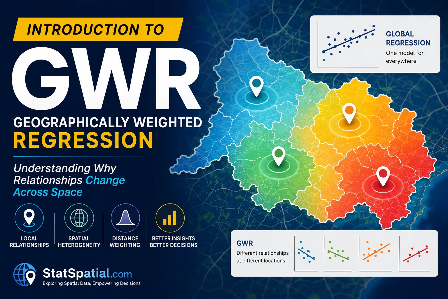
A traditional linear regression model estimates one global coefficient for each explanatory variable.

For example, $\text{House Price} = \beta_0 + \beta_1(\text{House Size})+\varepsilon$ House Price=β0+β1(House Size)+ε

Suppose the estimated coefficient is $\beta_1 = 2.5$ β1=2.5

This means that every additional square meter increases the house price by the same amount everywhere. However, in reality, the impact of house size may differ between urban and rural areas.

In a city center, one extra square meter may substantially increase the price.
In suburban areas, the effect may be moderate.
In rural regions, the increase may be relatively small.

A single global coefficient cannot capture these regional differences.

The Main Idea of GWR

Geographically Weighted Regression extends classical regression by allowing model coefficients to vary across locations. Instead of estimating one coefficient for the entire study area, GWR estimates a separate set of coefficients for every location. The model can be written as $y_i=\beta_0(u_i,v_i)+\sum_{k=1}^{p}\beta_k(u_i,v_i)x_{ik}+\varepsilon_i$ yi=β0(ui,vi)+k=1∑pβk(ui,vi)xik+εi

where

$u_i,v_i$ ui,vi are the geographic coordinates of location $i$ i,
each coefficient depends on location,
nearby observations have greater influence than distant observations.

In other words, GWR builds a local regression model at every location.

A Simple Example

Imagine we want to study how education affects household income in five districts.

District	Education (Years)	Income
A	9	Low
B	10	Low
C	12	Medium
D	15	High
E	15	Medium

A traditional regression estimates a single relationship between education and income. GWR, however, recognizes that local conditions differ. For example,

District	Local Effect of Education
A	Weak
B	Moderate
C	Moderate
D	Strong
E	Weak

Why? Because employment opportunities, industrial development, infrastructure, and local economic conditions vary from one district to another. Thus, education does not produce the same economic return everywhere.

How Does GWR Work?

The key concept behind GWR is distance-based weighting. When estimating the model for one location:

nearby observations receive large weights,
distant observations receive small weights.

A commonly used Gaussian kernel is $w_{ij}=\exp\left(-\frac{d_{ij}^{2}}{2h^{2}}\right)$ wij=exp(−2h2dij2)

where

$d_{ij}$ dij is the distance between locations $i$ i and $j$ j,
$h$ h is the bandwidth controlling how quickly weights decrease with distance.

This means that observations closer to the target location contribute more to the local regression than observations farther away.

Why Is Bandwidth Important?

The bandwidth determines the size of the local neighborhood.

Small bandwidth

Uses only nearby observations.
Captures detailed local variation.
May produce unstable estimates if too few observations are included.

Large bandwidth

Uses more observations.
Produces smoother coefficient estimates.
May overlook important local differences.

Choosing an appropriate bandwidth is therefore one of the most important steps in GWR.

Advantages of GWR

GWR offers several important benefits:

Captures spatial heterogeneity.
Produces location-specific parameter estimates.
Reveals spatial patterns hidden in global regression.
Helps identify regions where predictors have stronger or weaker effects.
Provides valuable insights for regional planning and policy-making.

Limitations of GWR

Although powerful, GWR is not suitable for every problem. Some challenges include:

higher computational cost than ordinary regression,
sensitivity to bandwidth selection,
possible multicollinearity among local predictors,
coefficients may become unstable when local sample sizes are small.

Researchers should therefore carefully evaluate model assumptions before applying GWR.

Applications of GWR

GWR has been widely applied in many fields, including:

poverty and socioeconomic studies,
housing price analysis,
environmental science,
epidemiology and public health,
transportation planning,
crime analysis,
agriculture,
urban and regional planning.

Whenever relationships are expected to vary geographically, GWR can provide more informative results than traditional regression.

Final Thoughts

Traditional regression assumes that one model fits every location. In many spatial problems, this assumption is too restrictive. Geographically Weighted Regression addresses this limitation by estimating local relationships, allowing coefficients to change across space. Instead of asking,

“What is the overall relationship?”

GWR asks,

“How does the relationship change from one place to another?”

This local perspective makes GWR an invaluable tool for understanding spatial processes and supporting evidence-based decision-making.