

Introduction
Similarity and Geographically Weighted Regression (SGWR) is a regression approach introduced by M. Naser Lessani and Zhenlong Li in their article “SGWR: Similarity and Geographically Weighted Regression.” This method integrates geographic proximity and attribute similarity within a local regression framework, referred to as SGWR.
The approach seeks to leverage the strengths of both concepts by capturing the complex interactions between spatial closeness and similarity in attributes, thereby providing a more robust understanding of spatial patterns.
According to Lessani and Li, geographic proximity and attribute similarity are not mutually exclusive; instead, they complement each other in determining the influence of one observation on another. By acknowledging this interaction, SGWR introduces a new way to conceptualize and operationalize “proximity,” extending it beyond purely spatial distance to include similarity across relevant attributes.
The article SGWR in this link https://doi.org/10.1080/13658816.2024.2342319
The Python packages for serial and parallel version of the model and also its Graphic User Interface (GUI) tool is available in this repository: https://github.com/Lessani252/FastSGWR
Data and Methods
The data is an Indonesian Human Development Index in 2024 of 38 Provinces from previous article.
y Human Development Index
x1 Gross Regional Domestic Product at Constant Prices (GRDP ADHK)
x2 Percentage of Households with Access to Adequate Sanitation by Province
x3 Prevalence of Insufficient Food Consumption (Percent)
x4 Average Percentage of Household Telecommunication Consumption to Total Consumption by Province
We would like to make a comparation between the two methods, the GWR from previous article and the SGWR in terms of AIC, R2.
Results and Discussions
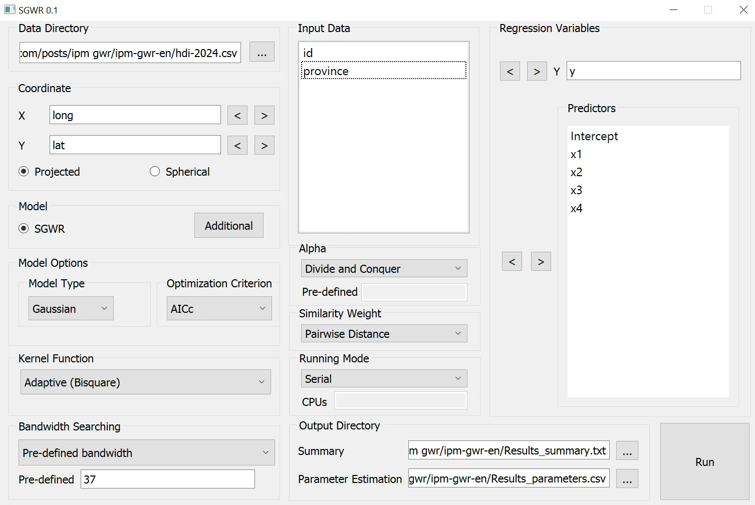
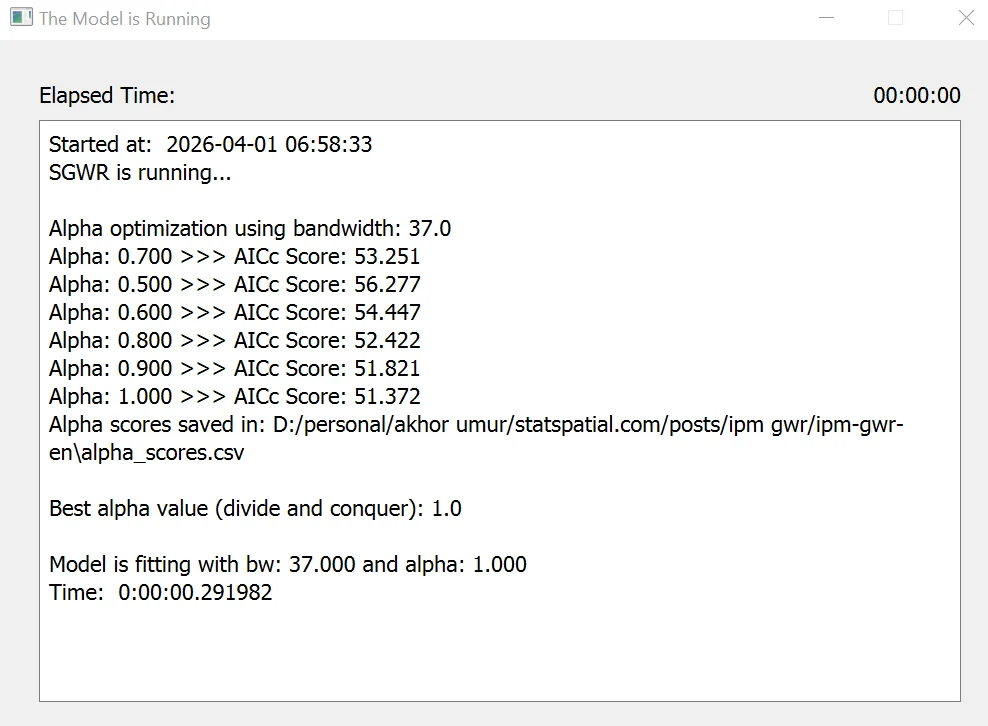
We doing the SGWR with GUI
================================================================================
SGWR Version: 0.1
Released Date: 04/25/2025
Development Team: M.Naser Lessani, Zhenlong Li,
Geoinformation and Big Data Research Laboratory (GIBD)
The Pennsylvania State University, University Park, PA, USA
================================================================================
Model type:                                                             Gaussian
Number of observations:                                                       38
Number of covariates:                                                          5
Dependent variable:                                                            y
Variable standardization:                                                     On
Total runtime:                                                           0:00:00

================================================================================
Global Regression Results
--------------------------------------------------------------------------------
Residual sum of squares:                                                   6.086
Log-likelihood:                                                          -19.118
AIC:                                                                      48.236
AICc:                                                                     52.946
R2:                                                                        0.840
Adj. R2:                                                                   0.820

Variable                                   Est.         SE  t(Est/SE)    p-value
------------------------------------ ---------- ---------- ---------- ----------
Intercept                                -0.000      0.070     -0.000      1.000
x1                                        0.243      0.075      3.230      0.001
x2                                        0.629      0.111      5.692      0.000
x3                                       -0.282      0.131     -2.152      0.031
x4                                        0.235      0.101      2.319      0.020

================================================================================
Similarity and Geographically Weighted Regression (SGWR) Results
--------------------------------------------------------------------------------
Coordinates type:                                                      Projected
Kernel Function:                                               Adaptive bisquare
Bandwidth optimization criterion:                                           AICc
Bandwidth used:                                                           37.000
--------------------------------------------------------------------------------

Diagnostic Information
--------------------------------------------------------------------------------
Residual sum of squares:                                                   4.799
Effective number of parameters (trace(S)):                                 7.353
Degree of freedom (n - trace(S)):                                         30.647
Sigma estimate:                                                            0.396
Log-likelihood:                                                          -14.606
Degree of Dependency (DoD):                                                0.894
AIC:                                                                      45.918
AICc:                                                                     51.372
BIC:                                                                      59.596
R2:                                                                        0.874
Adj. R2:                                                                   0.842
Adj. alpha (95%):                                                          0.034
Adj. critical t value (95%):                                               2.202
Weight combination (alpha):                                                1.000
Mean Absolute Percentage Error:                                           75.821
Mean Absolute Error:                                                       0.277
Root Mean Squared Error:                                                   0.355
--------------------------------------------------------------------------------

Summary Statistics For SGWR Parameter Estimates
--------------------------------------------------------------------------------
Variable                        Mean        STD        Min     Median        Max
--------------------      ---------- ---------- ---------- ---------- ----------
Intercept                     -0.065      0.047     -0.130     -0.086      0.023
x1                             0.251      0.014      0.223      0.259      0.265
x2                             0.749      0.071      0.666      0.728      0.892
x3                            -0.279      0.080     -0.383     -0.291     -0.148
x4                             0.283      0.071      0.154      0.325      0.355
================================================================================
The output results compare the Global Regression (Standard) and the SGWR (Local) models. Overall, the SGWR model is superior in explaining the data because it successfully captures inter-regional variations.
1. Model Performance (Global vs. Local)
The SGWR model outperforms the Global Regression model based on the following statistical indicators:
- Accuracy (R2): Increased from 0.840 (Global) to 0.874 (SGWR). This means the local model can explain 87.4% of the variation in the dependent variable (y).
- AICc: Decreased from 52.946 to 51.372. In statistics, a lower AICc value indicates a more efficient model that better fits reality.
- RSS (Residuals): The Residual Sum of Squares decreased from 6.086 to 4.799, indicating that the local model’s predictions are more accurate.
2. Global Significance Analysis
In the Global model, all independent variables (x1, x2, x3, x4) have a p-value < 0.05, meaning all of them have a significant impact on y as a national average. x2 has the largest positive influence (Coefficient: 0.629). x3 is the only variable with a negative influence (Coefficient: -0.282).
3. Spatial Variation (SGWR Results)
This is the most critical part. SGWR shows that the influence of each variable varies by location (it is not uniform):
- Bandwidth (37,000): Indicates the spatial reach used to calculate local estimates.
- Coefficient Range (Min to Max):
- x2: Its influence ranges from 0.666 to 0.892. In some regions, x2 is highly dominant, while in others, its influence is more moderate.
- x4: Shows a fairly wide variation (Min: 0.154, Max: 0.355). This proves the existence of spatial non-stationarity—policies or x4 factors might be very effective in one province but less so in a neighboring one.
- x1: Tends to be more stable across all regions (STD: 0.014).
The GWR method from previous article shows the following result:
   ***********************************************************************
   *                       Package   GWmodel                             *
   ***********************************************************************
   Program starts at: 2026-03-31 22:11:23.629035
   Call:
   gwr.basic(formula = y ~ x1 + x2 + x3 + x4, data = data_sp, bw = bw_opt,
    kernel = "bisquare", adaptive = TRUE)

   Dependent (y) variable:  y
   Independent variables:  x1 x2 x3 x4
   Number of data points: 38
   ***********************************************************************
   *                    Results of Global Regression                     *
   ***********************************************************************

   Call:
    lm(formula = formula, data = data)

   Residuals:
    Min      1Q  Median      3Q     Max
-4.7905 -0.9212 -0.2494  1.0178  5.2864

   Coefficients:
                 Estimate Std. Error t value Pr(>|t|)
   (Intercept)  4.687e+01  3.403e+00  13.774 3.08e-15 ***
   x1           2.366e-06  7.326e-07   3.230   0.0028 **
   x2           2.150e-01  3.778e-02   5.692 2.39e-06 ***
   x3          -1.639e-01  7.613e-02  -2.152   0.0388 *
   x4           2.484e+00  1.071e+00   2.319   0.0267 *

   ---Significance stars
   Signif. codes:  0 '***' 0.001 '**' 0.01 '*' 0.05 '.' 0.1 ' ' 1
   Residual standard error: 2.182 on 33 degrees of freedom
   Multiple R-squared: 0.8399
   Adjusted R-squared: 0.8204
   F-statistic: 43.27 on 4 and 33 DF,  p-value: 1.113e-12
   ***Extra Diagnostic information
   Residual sum of squares: 157.1707
   Sigma(hat): 2.089462
   AIC:  173.7897
   AICc:  176.4994
   BIC:  167.4407
   ***********************************************************************
   *          Results of Geographically Weighted Regression              *
   ***********************************************************************

   *********************Model calibration information*********************
   Kernel function: bisquare
   Adaptive bandwidth: 37 (number of nearest neighbours)
   Regression points: the same locations as observations are used.
   Distance metric: Euclidean distance metric is used.

   ****************Summary of GWR coefficient estimates:******************
                    Min.     1st Qu.      Median     3rd Qu.    Max.
   Intercept  3.2529e+01  3.7222e+01  4.0339e+01  4.2192e+01 47.3504
   x1         2.1854e-06  2.2949e-06  2.5013e-06  2.5666e-06  0.0000
   x2         2.3003e-01  2.4239e-01  2.5879e-01  2.8456e-01  0.3310
   x3        -2.2405e-01 -2.1244e-01 -1.7582e-01 -1.1610e-01 -0.0811
   x4         1.5593e+00  2.5316e+00  3.4406e+00  3.5718e+00  3.7137
   ************************Diagnostic information*************************
   Number of data points: 38
   Effective number of parameters (2trace(S) - trace(S'S)): 8.761736
   Effective degrees of freedom (n-2trace(S) + trace(S'S)): 29.23826
   AICc (GWR book, Fotheringham, et al. 2002, p. 61, eq 2.33): 175.5039
   AIC (GWR book, Fotheringham, et al. 2002,GWR p. 96, eq. 4.22): 160.2578
   BIC (GWR book, Fotheringham, et al. 2002,GWR p. 61, eq. 2.34): 142.1247
   Residual sum of squares: 123.8168
   R-square value:  0.873839
   Adjusted R-square value:  0.8346939

   ***********************************************************************
   Program stops at: 2026-03-31 22:11:23.710312
COMPARISON ANALYSIS
Methods     bandwidth    AIC         R-square     RSS
SGWR          37         45.918      0.874        4.799
GWR           37         160.2578    0.873839     123.8168
The table compares the performance of SGWR (Similarity and Geographically Weighted Regression) against the standard GWR (Geographically Weighted Regression). Although both models use the same bandwidth (37), their statistical efficiency differs significantly.
- Model Accuracy (R-square): Both models show very high and nearly identical explanatory power, with SGWR at 0.874 and GWR at 0.8738. This indicates that both models can account for approximately 87.4% of the variation in the dependent variable.
- Statistical Efficiency (AIC): SGWR is significantly more efficient than GWR. The AIC for SGWR (45.918) is much lower than that of GWR (160.257). In model selection, a lower AIC indicates a better fit with less complexity (parsimony).
- Error Minimization (RSS): SGWR is vastly superior in terms of precision. Its Residual Sum of Squares (RSS) is only 4.799, whereas GWR has a much higher error rate of 123.816. This suggests that SGWR’s integration of “similarity” weighting significantly reduces prediction errors compared to a purely geographical approach.
CONCLUSION
While both models capture spatial non-stationarity effectively, SGWR is the superior model. It achieves a similar R-square but with a drastically lower AIC and RSS, proving it is more reliable and precise for this specific dataset.


