

The processing steps done from previous articles: article-1 and article-2 are:
- Importing the data of HDI into R
- Importing the provincial shapefile and HDI dataset into R.
- Doing the statistics descriptive with histogram etc.
- Merging attribute data with spatial geometries using a left join operation.
Doing the Linear Regression OLS model - Multicolinearity test, Normality test, Heteroscedasticity test, Non autocorrelation test
In this article, we continue the steps until finish:
- GWR Modelling
- Plotting the coefficients, the coefficients t-value, the y estimation, the residual
- Interpretations
Results and Discussions
GWR MODELING
A. Preparing Spatial Data: GWmodel does not use the sf format directly, but rather a SpatialPointsDataFrame (sp format). We must first convert the provincial polygons to centroids.
Make sure the CRS (coordinate system) is projected in meters, not degrees.
Example: UTM Zone 48S for most of Indonesia (EPSG: 23848)
map_prov_hdi_st <- st_transform(map_prov_hdi, 23848)Take the center point (centroid) of the province
coords <- st_centroid(map_prov_hdi_st)Convert to spatial format (Here’s the solution). The ‘as’ function will automatically convert the sf object to a SpatialPointsDataFrame.
data_sp <- as(coords, "Spatial")
data_sp

result:
class       : SpatialPointsDataFrame
features    : 38
extent      : -401491, 4578050, -1072345, 472469.3  (xmin, xmax, ymin, ymax)
crs         : +proj=utm +zone=48 +a=6378160 +rf=298.247 +units=m +no_defs
variables   : 11
names       :   id, KODE_PROV,       PROVINSI,       province,     y,         x1,    x2,    x3,   x4,         lat,        long
min values  :   11,        11,           Aceh,           ACEH, 53.42,   13798.74, 12.61,  2.55, 2.58, -10.1712931,  95.3353979
max values  : 92-B,        92, Sumatera Utara, SUMATERA UTARA, 83.08, 2151198.76, 96.83, 37.69, 4.69,   5.5698054, 140.7120414
Now data_sp can be entered into the GWR model. Check if the coordinates are readable.
print(proj4string(data_sp))

result:
[1] "+proj=utm +zone=48 +a=6378160 +rf=298.247 +units=m +no_defs"
B. Finding the Optimal BandwidthBandwidth is the “view distance” of the model. If it is too small, the model is too volatile (overfit). If it is too large, the model becomes equivalent to global OLS. Use the AICc criterion to find the best bandwidth.
bw_opt <- bw.gwr(y ~ x1+x2+x3+x4,
                 data = data_sp,
                 approach = "AICc",
                 adaptive = TRUE)
cat("Optimum bandwidth:", bw_opt, "\n")

result:
Adaptive bandwidth (number of nearest neighbours): 31 AICc value: 178.6269
Adaptive bandwidth (number of nearest neighbours): 27 AICc value: 182.8606
Adaptive bandwidth (number of nearest neighbours): 34 AICc value: 177.0428
Adaptive bandwidth (number of nearest neighbours): 35 AICc value: 176.2125
Adaptive bandwidth (number of nearest neighbours): 37 AICc value: 175.5039
Adaptive bandwidth (number of nearest neighbours): 37 AICc value: 175.5039
Optimum bandwidth: 37
C. Running the GWR Model (Level-2) After bw_opt is obtained, we enter it into the gwr.basic.R# function Run GWR
gwr_ipm <- gwr.basic(y ~ x1+x2+x3+x4, data = data_sp,bw = bw_opt,adaptive = TRUE,kernel = "bisquare")
print(gwr_ipm)

result:
   ***********************************************************************
   *                       Package   GWmodel                             *
   ***********************************************************************
   Program starts at: 2026-03-31 22:11:23.629035
   Call:
   gwr.basic(formula = y ~ x1 + x2 + x3 + x4, data = data_sp, bw = bw_opt,
    kernel = "bisquare", adaptive = TRUE)

   Dependent (y) variable:  y
   Independent variables:  x1 x2 x3 x4
   Number of data points: 38
   ***********************************************************************
   *                    Results of Global Regression                     *
   ***********************************************************************

   Call:
    lm(formula = formula, data = data)

   Residuals:
    Min      1Q  Median      3Q     Max
-4.7905 -0.9212 -0.2494  1.0178  5.2864

   Coefficients:
                 Estimate Std. Error t value Pr(>|t|)
   (Intercept)  4.687e+01  3.403e+00  13.774 3.08e-15 ***
   x1           2.366e-06  7.326e-07   3.230   0.0028 **
   x2           2.150e-01  3.778e-02   5.692 2.39e-06 ***
   x3          -1.639e-01  7.613e-02  -2.152   0.0388 *
   x4           2.484e+00  1.071e+00   2.319   0.0267 *

   ---Significance stars
   Signif. codes:  0 '***' 0.001 '**' 0.01 '*' 0.05 '.' 0.1 ' ' 1
   Residual standard error: 2.182 on 33 degrees of freedom
   Multiple R-squared: 0.8399
   Adjusted R-squared: 0.8204
   F-statistic: 43.27 on 4 and 33 DF,  p-value: 1.113e-12
   ***Extra Diagnostic information
   Residual sum of squares: 157.1707
   Sigma(hat): 2.089462
   AIC:  173.7897
   AICc:  176.4994
   BIC:  167.4407
   ***********************************************************************
   *          Results of Geographically Weighted Regression              *
   ***********************************************************************

   *********************Model calibration information*********************
   Kernel function: bisquare
   Adaptive bandwidth: 37 (number of nearest neighbours)
   Regression points: the same locations as observations are used.
   Distance metric: Euclidean distance metric is used.

   ****************Summary of GWR coefficient estimates:******************
                    Min.     1st Qu.      Median     3rd Qu.    Max.
   Intercept  3.2529e+01  3.7222e+01  4.0339e+01  4.2192e+01 47.3504
   x1         2.1854e-06  2.2949e-06  2.5013e-06  2.5666e-06  0.0000
   x2         2.3003e-01  2.4239e-01  2.5879e-01  2.8456e-01  0.3310
   x3        -2.2405e-01 -2.1244e-01 -1.7582e-01 -1.1610e-01 -0.0811
   x4         1.5593e+00  2.5316e+00  3.4406e+00  3.5718e+00  3.7137
   ************************Diagnostic information*************************
   Number of data points: 38
   Effective number of parameters (2trace(S) - trace(S'S)): 8.761736
   Effective degrees of freedom (n-2trace(S) + trace(S'S)): 29.23826
   AICc (GWR book, Fotheringham, et al. 2002, p. 61, eq 2.33): 175.5039
   AIC (GWR book, Fotheringham, et al. 2002,GWR p. 96, eq. 4.22): 160.2578
   BIC (GWR book, Fotheringham, et al. 2002,GWR p. 61, eq. 2.34): 142.1247
   Residual sum of squares: 123.8168
   R-square value:  0.873839
   Adjusted R-square value:  0.8346939

   ***********************************************************************
   Program stops at: 2026-03-31 22:11:23.710312
Comparing AIC
data.frame("MODEL" = c("GWR","OLS"),
           "AIC" = c(gwr_ipm$GW.diagnostic$AIC,AIC(ipmlm)),
           "R2" = c(gwr_ipm$GW.diagnostic$gw.R2,summary(ipmlm)$r.squared))%>% arrange(AIC)

result:
Model   AIC             R2
GWR	160.2578	0.8738390
OLS	173.7897	0.8398536
2 rows
MERGING GWR RESULT WITH MAP_PROV_HDI
First, check the order of values whether they are the same, if they are the same they will be combined.
all.equal(gwr_ipm$SDF$y, map_prov_hdi$y)
result:
1] TRUE
results2 <-as.data.frame(gwr_ipm$SDF)
gwr.map <- cbind(map_prov_hdi, as.matrix(results2))
gwr.mapPLOTTING LOCAL-R2
#initializing the library for plot using tmap
library(tmap)
qtm(gwr.map, fill = "Local_R2")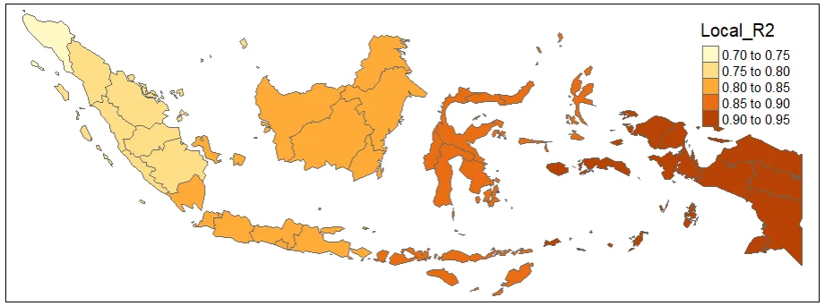
PLOTTING Y_HAT
#Spatial distribution of yhat
map_yhat <- tm_shape(gwr.map2) +
  tm_fill("yhat",
          n = 5,
          style = "quantile",
          title = "Y hat")  +
  tm_borders(col = "black", lwd = 0.5)+
  tm_layout(frame = FALSE,
            legend.text.size = 0.5,
            legend.title.size = 0.6)
map_yhat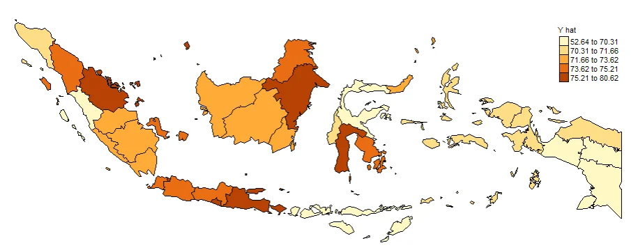
PLOTTING THE COEFFICIENTS
The purpose of GWR is to observe how the relationship between variables changes spatially. Therefore, the most important to show are Local Coefficients (local β).
Example: x1, x2, x3, x4
This is the core of GWR with the Interpretation: Positive / negative, Strong / weak, Differs between provinces.
#Spatial distribution of Intercept
map0 <- tm_shape(gwr.map2) +
  tm_fill("Intercept",
          n = 5,
          style = "quantile",
          title = "Intercept")  +
  tm_borders(col = "black", lwd = 0.5)+
  tm_layout(frame = FALSE,
            legend.text.size = 0.5,
            legend.title.size = 0.6)
map0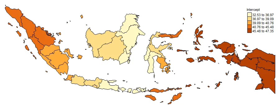
#Spatial distribution of x1
map1 <- tm_shape(gwr.map2) +
  tm_fill("x1",
          n = 5,
          style = "quantile",
          title = "x1 Gross Regional Domestic Product")  +
  tm_borders(col = "black", lwd = 0.5)+
  tm_layout(frame = FALSE,
            legend.text.size = 0.5,
            legend.title.size = 0.6)
map1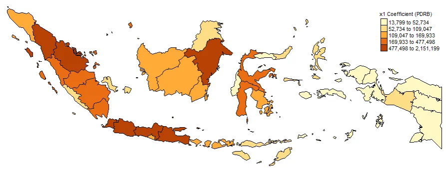
#Spatial distribution of x2
map2 <- tm_shape(gwr.map2) +
  tm_fill("x2",
          n = 5,
          style = "quantile",
          title = "x2 Coefficient (Adequate Sanitation)")  +
  tm_borders(col = "black", lwd = 0.5)+
  tm_layout(frame = FALSE,
            legend.text.size = 0.5,
            legend.title.size = 0.6)
map2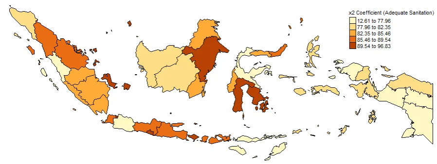
#Spatial distribution of x3
map3 <- tm_shape(gwr.map2) +
  tm_fill("x3",
          n = 5,
          style = "quantile",
          title = "x3 Prevalence of Insufficient Food Consumption")  +
  tm_borders(col = "black", lwd = 0.5)+
  tm_layout(frame = FALSE,
            legend.text.size = 0.5,
            legend.title.size = 0.6)
map3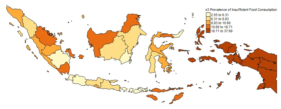
#Spatial distribution of x4
map4 <- tm_shape(gwr.map2) +
  tm_fill("x4",
          n = 5,
          style = "quantile",
          title = "x4 Telecommunication Consumption")  +
  tm_borders(col = "black", lwd = 0.5)+
  tm_layout(frame = FALSE,
            legend.text.size = 0.5,
            legend.title.size = 0.6)
map4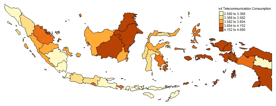
PLOTTING COEFFICIENTS T-VALUE
Plotting T-value (TV) is important. Intercept_TV, x1_TV, x2_TV, x3_TV, x4_TV. These are used to determine whether or not a value is significant at each location. Often used to create significance maps. The larger the value indicates that the coefficient is more significant in that province.
#Spatial distribution of Intercept t-value
map0_TV <- tm_shape(gwr.map2) +
  tm_fill("Intercept_TV",
          n = 5,
          style = "quantile",
          title = "Intercept t-value")  +
  tm_borders(col = "black", lwd = 0.5)+
  tm_layout(frame = FALSE,
            legend.text.size = 0.5,
            legend.title.size = 0.6)
map0_TV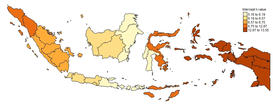
#Spatial distribution of x1 t-value
map1_TV <- tm_shape(gwr.map2) +
  tm_fill("x1_TV",
          n = 5,
          style = "quantile",
          title = "x1 t-value")  +
  tm_borders(col = "black", lwd = 0.5)+
  tm_layout(frame = FALSE,
            legend.text.size = 0.5,
            legend.title.size = 0.6)
map1_TV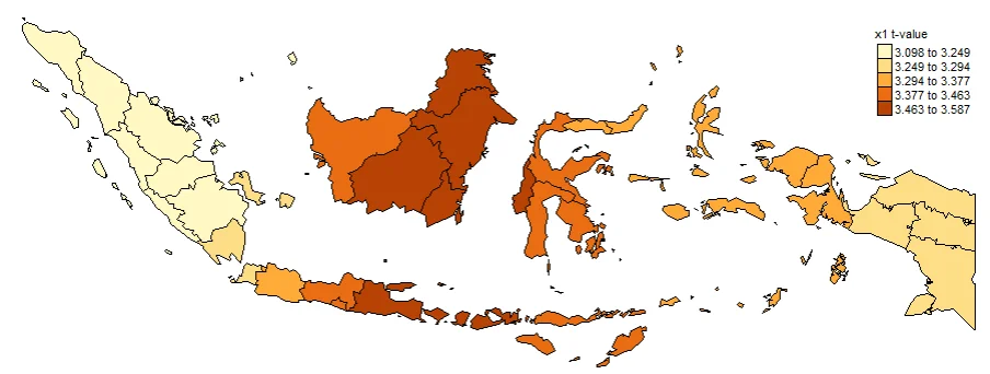
#Spatial distribution of x2 t-value
map2_TV <- tm_shape(gwr.map2) +
  tm_fill("x2_TV",
          n = 5,
          style = "quantile",
          title = "x2 t-value")  +
  tm_borders(col = "black", lwd = 0.5)+
  tm_layout(frame = FALSE,
            legend.text.size = 0.5,
            legend.title.size = 0.6)
map2_TV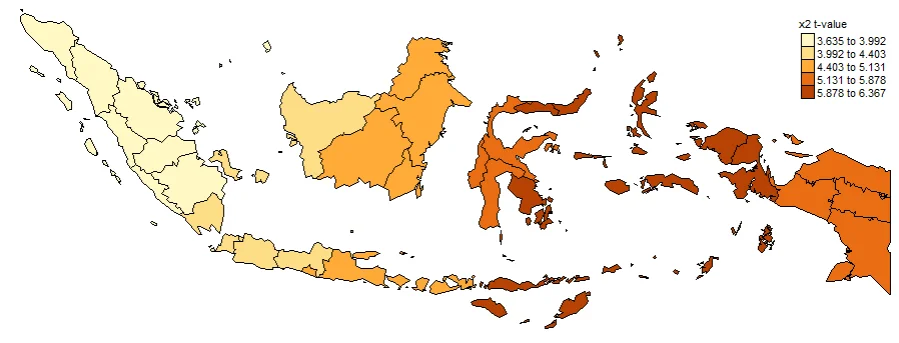
#Spatial distribution of x3 t-value
map3_TV <- tm_shape(gwr.map2) +
  tm_fill("x3_TV",
          n = 5,
          style = "quantile",
          title = "x3 t-value")  +
  tm_borders(col = "black", lwd = 0.5)+
  tm_layout(frame = FALSE,
            legend.text.size = 0.5,
            legend.title.size = 0.6)
map3_TV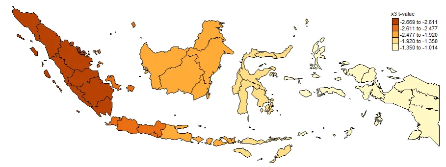
#Spatial distribution of x4 t-value
map4_TV <- tm_shape(gwr.map2) +
  tm_fill("x4_TV",
          n = 5,
          style = "quantile",
          title = "x4 t-value")  +
  tm_borders(col = "black", lwd = 0.5)+
  tm_layout(frame = FALSE,
            legend.text.size = 0.5,
            legend.title.size = 0.6)
map4_TV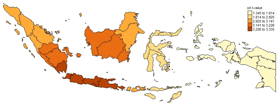
PLOTTING RESIDUAL
Plotting Residuals is also important thing to do. It used to see Overestimated areas and Underestimated areas. It also important for Model diagnosis. The closer the residual value is to zero, the more accurate the estimate of the y value is. If the residual value is negative, it is an underestimation, and if the residual value is positive, it is an underestimation.
#Spatial distribution of residual
map_residual <- tm_shape(gwr.map2) +
  tm_fill("residual",
          n = 5,
          style = "quantile",
          title = "Residual",
          midpoint = NA)  +
  tm_borders(col = "black", lwd = 0.5)+
  tm_shape(st_centroid(gwr.map2)) +
  tm_text(
    # The key argument: specify the column for the text labels
    text = "id",
    # Optional arguments to customize the text appearance
    size = 0.8,
    #fontface = "bold",
    col = "black",
    shadow = FALSE
  ) +
  tm_layout(frame = FALSE,
            legend.text.size = 0.5,
            legend.title.size = 0.6)
map_residual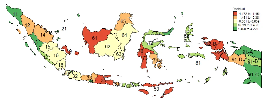
id province
11 ACEH
12 SUMATERA UTARA
13 SUMATERA BARAT
14 RIAU
15 JAMBI
16 SUMATERA SELATAN
17 BENGKULU
18 LAMPUNG
19 KEP. BANGKA BELITUNG
21 KEP. RIAU
31 DKI JAKARTA
32 JAWA BARAT
33 JAWA TENGAH
34 DI YOGYAKARTA
35 JAWA TIMUR
36 BANTEN
51 BALI
52 NUSA TENGGARA BARAT
53 NUSA TENGGARA TIMUR
61 KALIMANTAN BARAT
62 KALIMANTAN TENGAH
63 KALIMANTAN SELATAN
64 KALIMANTAN TIMUR
65 KALIMANTAN UTARA
71 SULAWESI UTARA
72 SULAWESI TENGAH
73 SULAWESI SELATAN
74 SULAWESI TENGGARA
75 GORONTALO
76 SULAWESI BARAT
81 MALUKU
82 MALUKU UTARA
92-A PAPUA BARAT
92-B PAPUA BARAT DAYA
91-A PAPUA
91-C PAPUA SELATAN
91-D PAPUA TENGAH
91-B PAPUA PEGUNUNGAN


