


Introduction
The Human Development Index (HDI) is a widely used composite indicator for assessing the overall level of human development in a region. It reflects achievements in three fundamental dimensions of human well-being: health, education, and standard of living. By integrating these dimensions into a single index, HDI provides a comprehensive measure that goes beyond purely economic indicators and captures broader aspects of social development.
This article aims to visualize the 2024 Human Development Index, Coefficients, Residual, HDI estimation, Coefficient Significations across all provinces in Indonesia using the R programming language. The resulting visualization is expected to support exploratory analysis of spatial disparities in human development and serve as a useful reference for researchers, students, and policymakers interested in regional development analysis in Indonesia. This study utilizes provincial-level Human Development Index (HDI) data for the year 2024 published by Central Statistics Agency (Badan Pusat Statistik, BPS).
Data Structure
y Human Development Index
x1 Gross Regional Domestic Product at Constant Prices (GRDP ADHK)
x2 Percentage of Households with Access to Adequate Sanitation by Province
x3 Prevalence of Insufficient Food Consumption (Percent)
x4 Average Percentage of Household Telecommunication Consumption to Total Consumption by Province
The data is at province level from all provinces in Indonesia (38 Provinces).
Data, R codes and materials can be obtained here.
Methods
The processing steps included:
- Importing the data of HDI into R
- Importing the provincial shapefile and HDI dataset into R.
- Doing the statistics descriptive with histogram etc.
- Merging attribute data with spatial geometries using a left join operation.
- Doing the Linear Regression OLS model
- Multicolinearity test, Normality test, Heteroscedasticity test, Non autocorrelation test
- GWR Modelling
- Plotting the coefficients, the coefficients t-value, the y estimation, the residual
- Interpretations
Results and Discussions
We analize the data using GWR methods in R.
#initializing libraries
library(readxl)
library(tidyverse)
library(ggplot2)
library(sp)
library(sf)
library(spgwr)
library(spdep)
library(spData)
library(GWmodel)
hdi <- read_excel("D:/personal/akhor umur/statspatial.com/posts/ipm gwr/ipm-gwr-en/hdi 2024.xlsx")
hdi
str(hdi)
hdi1<-hdi%>% dplyr::select(y,x1,x2,x3,x3,x4)
str(hdi1)
tibble [38 × 5] (S3: tbl_df/tbl/data.frame) $ y : num [1:38] 74 74 74.5 74.8 73.4 ... $ x1: num [1:38] 153780 632535 199420 571234 176868 ... $ x2: num [1:38] 81.1 85.7 72.8 86.3 84 ... $ x3: num [1:38] 9.1 7.54 8.88 10.93 10.58 ... $ x4: num [1:38] 3.27 3.55 3.59 3.95 3.66 3.29 3.62 3.28 3.6 4 ...
plot_histogram(hdi1)

plot_boxplot(hdi1,by="y")

library(GGally)
ggcorr(hdi1, label = TRUE, label_size = 2.9, hjust = 1, layout.exp = 5)

Interpretations:
Correlation with y (response variable)
- y – x2 = 0.9 → 🔴 Very strong positive correlation
x2 is the most influential variable on y (strong direct relationship) - y – x3 = -0.6 → 🔵 Moderately strong negative correlation
As x3 increases, y tends to decrease - y – x1 = 0.4 → 🟠 Moderate positive correlation
x1 has some effect, but not dominant - y – x4 = 0.1 → ⚪ Very weak correlation
Almost no relationship with y
Correlation among independent variables
- x2 – x3 = -0.6 → 🔵 Moderately strong negative correlation
Indicates an inverse relationship - x3 – x4 = 0.5 → 🟠 Moderate positive correlation
Potential mild multicollinearity - x1 – x3 = -0.4 → 🔵 Moderate negative correlation
- x1 – x4 = -0.3 → 🔵 Weak to moderate negative correlation
- x1 – x2 = 0.2 → ⚪ Weak correlation
- x2 – x4 = 0.1 → ⚪ Very weak correlation
Next Importing the map shp file into R :
library(spdep)
library(sf)
map_prov<- st_read(file.path("D:/ipm-gwr/shp_prov38_geojson.shp"))
print(map_prov)

result:
Reading layer `shp_prov38_geojson' from data source
`D:\personal\akhor umur\statspatial.com\posts\ipm gwr\shp_prov38_geojson\shp_prov38_geojson.shp' using driver `ESRI Shapefile'
Simple feature collection with 38 features and 3 fields
Geometry type: MULTIPOLYGON
Dimension: XY
Bounding box: xmin: 95.19355 ymin: -10.93017 xmax: 141.02 ymax: 5.907129
Geodetic CRS: WGS 84
Simple feature collection with 38 features and 3 fields
Geometry type: MULTIPOLYGON
Dimension: XY
Bounding box: xmin: 95.19355 ymin: -10.93017 xmax: 141.02 ymax: 5.907129
Geodetic CRS: WGS 84
First 10 features:
id KODE_PROV PROVINSI geometry
1 72 72 Sulawesi Tengah MULTIPOLYGON (((119.5612 -0...
2 76 76 Sulawesi Barat MULTIPOLYGON (((119.5612 -0...
3 73 73 Sulawesi Selatan MULTIPOLYGON (((120.9238 -7...
4 91-D 91 Papua Tengah MULTIPOLYGON (((134.8855 -4...
5 92-A 92 Papua Barat MULTIPOLYGON (((133.3384 -4...
6 75 75 Gorontalo MULTIPOLYGON (((121.3367 0....
7 14 14 Riau MULTIPOLYGON (((100.1812 0....
8 91-C 91 Papua Selatan MULTIPOLYGON (((138.8213 -8...
9 34 34 Daerah Istimewa Yogyakarta MULTIPOLYGON (((110.0035 -7...
10 13 13 Sumatera Barat MULTIPOLYGON (((99.27609 -1...
#check if map is valid
table(st_geometry_type(map_prov))
sum(st_is_empty(map_prov))
sum(!st_is_valid(map_prov))

result:
          GEOMETRY              POINT         LINESTRING            POLYGON         MULTIPOINT    MULTILINESTRING       MULTIPOLYGON
                 0                  0                  0                  0                  0                  0                 38
GEOMETRYCOLLECTION     CIRCULARSTRING      COMPOUNDCURVE       CURVEPOLYGON         MULTICURVE       MULTISURFACE              CURVE
                 0                  0                  0                  0                  0                  0                  0
           SURFACE  POLYHEDRALSURFACE                TIN           TRIANGLE
                 0                  0                  0                  0
[1] 0
[1] 2
#validate the map
sf_use_s2(FALSE)
map_prov<- map_prov|> st_make_valid()#check again if the map is valid
sum(!st_is_valid(map_prov))
result:
[1] 0
[1] 0Join the map with data hdi 2024 by column ‘id’:
map_prov_hdi <- map_prov %>%
left_join(hdi, by = "id")
print(map_prov_hdi)
result:
Simple feature collection with 38 features and 11 fields
Geometry type: MULTIPOLYGON
Dimension: XY
Bounding box: xmin: 95.19355 ymin: -10.93017 xmax: 141.02 ymax: 5.907129
Geodetic CRS: WGS 84
First 10 features:
id KODE_PROV PROVINSI province y x1 x2 x3 x4 lat long
1 72 72 Sulawesi Tengah SULAWESI TENGAH 71.56 212281.54 77.40 10.51 3.68 -0.8905452 119.8684
2 76 76 Sulawesi Barat SULAWESI BARAT 68.20 37088.74 82.52 6.53 3.50 -2.6649887 118.8502
3 73 73 Sulawesi Selatan SULAWESI SELATAN 74.05 396141.74 93.83 6.99 3.50 -5.1391049 119.4498
4 91-D 91 Papua Tengah PAPUA TENGAH 59.75 105472.48 41.44 37.69 4.08 -3.3669086 135.4952
5 92-A 92 Papua Barat PAPUA BARAT 67.02 49486.23 79.00 21.91 4.60 -0.9182756 134.0279
6 75 75 Gorontalo GORONTALO 71.23 32951.94 82.99 15.99 3.38 0.5238415 123.0749
7 14 14 Riau RIAU 74.79 571233.59 86.32 10.93 3.95 0.5176961 101.4433
8 91-C 91 Papua Selatan PAPUA SELATAN 67.90 19061.51 60.85 29.26 4.48 -8.4818571 140.3878
9 34 34 Daerah Istimewa Yogyakarta DI YOGYAKARTA 81.55 124590.45 96.71 9.05 3.94 -7.7950578 110.3671
10 13 13 Sumatera Barat SUMATERA BARAT 74.49 199419.96 72.82 8.88 3.59 -0.9376307 100.3578
geometry
1 MULTIPOLYGON (((119.5612 -0...
2 MULTIPOLYGON (((119.5612 -0...
3 MULTIPOLYGON (((120.9238 -7...
4 MULTIPOLYGON (((134.8855 -4...
5 MULTIPOLYGON (((133.3384 -4...
6 MULTIPOLYGON (((121.3367 0....
7 MULTIPOLYGON (((100.1812 0....
8 MULTIPOLYGON (((138.8213 -8...
9 MULTIPOLYGON (((110.0035 -7...
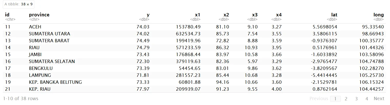
10 MULTIPOLYGON (((99.27609 -1...Now we create map plot for each variable to show how the variables are different in each province.
library(ggspatial)
# create function to make a map for every variable
plot_variable <- function(data, variable, title) {
ggplot() +
  geom_sf(
    data = map_prov,
    aes(fill = variable),
    color = "grey30",
    linewidth = 0.2
  ) +

  scale_fill_gradient(
    low = "#FFF400",
    high = "#D10000",
    name = "Values"
  ) +

  labs(
    title = title,
    #caption = "source: BPS",
    size = 0.3
  ) +

  theme_minimal() +
  theme(
    panel.grid = element_blank(),
    plot.title = element_text(face = "bold", size = 10)
  )
}

plot_y <- plot_variable(map_prov_hdi, map_prov_hdi$y, "HDI Distribution in Indonesia")
plot_y
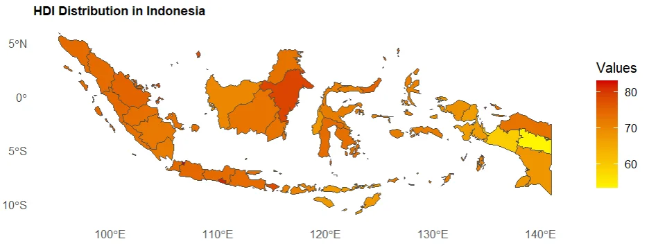
# Plot the predictors variables
plot_x1 <- plot_variable(map_prov_hdi, map_prov_hdi$x1, "Gross Regional Domestic Product \nAt Constant Prices")
plot_x2 <- plot_variable(map_prov_hdi, map_prov_hdi$x2, "Percentage of Households Having \nAccess to Sanitation")
plot_x3 <- plot_variable(map_prov_hdi, map_prov_hdi$x3, "Prevalence of Insufficient Food \nConsumption")
plot_x4 <- plot_variable(map_prov_hdi, map_prov_hdi$x4, "Average Percentage of Household \nTelecommunication Consumption \nto Total Consumption")

library(gridExtra)
grid.arrange(plot_x1, plot_x2, plot_x3, plot_x4, ncol = 2, widths = c(3, 3))
Continue to Geographically Weighted Regression on Indonesian Human Development Index in 2024 (Part 2).


